
my colour short course is
now offered online through
Australia's National Art
School in Sydney! There's
a choice of two sessions to
suit every time zone. LINK
Home
The Dimensions of Colour
Basics of Light and Shade
Basics of Colour Vision
Additive Mixing
Subtractive Mixing
Hue
Lightness and Chroma
Brightness and Saturation
Principles of Colour
Afterthoughts
Glossary
References
Contact
Links
NEXT COLOUR
WORKSHOPS

5.3 SUBTRACTIVE COMPLEMENTARIES
Subtractive vs additive complementaries
We've seen that the term "complementary" in additive mixing refers to colours of pairs of lights that mix to make white light. This white light may be seen as white light, or in the case of optical mixing, as a white or a grey object colour. In subtractive mixing, "complementary" also refers to pairs of colours that produce a neutral mixture, which is usually seen as a grey or a black object colour.
The subtractive complementary of a colour is frequently not the same as its additive complementary, even in the relatively simple case of subtractive mixing of digital colours. Consider an RGB colour with linear (i.e. energy-proportional) RGB of a b c, where a,b, and c are expressed as fractions of the maximum R, G and B respectively. Additive complementaries of abc would include the RGB colour 1-a 1-b 1-c, plus all colours differing from this only in brightness and/or saturation (that is, all colours of the same hue angle). Subtractive complementaries of abc however would include all colours with R,G and B in the ratio 1/a: 1/b:1/c, because these would multiply with abc to give a neutral result; this set of colours would have a common hue angle and saturation, but would vary in brightness.
As an example (Fig. 5.3.1), consider a purple with linear RGB of 0.60 0.20 1.00 (or 153 051 255), and a green with linear RGB of 0.40 0.80 0.00 (or 102 204 000). These two colours are additive complementaries because they can combine (in the right proportions) to make white light, as would be any other pair of RGB colours of the same two hue angles. They are not subtractive complementaries however, because they would not multiply to bring all three components of the purple colour to the same level. A green that would do this is one with linear RGB of 0.33, 1.00, 0.20 (or 085 255 051).
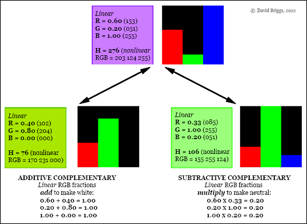
Figure 5.3.1. Additive and subtractive complementaries of a single colour differing in hue angle by 30°. The additive complementary adds to make white light; the subtractive complementary multiplies the R,G and B brightnesses to make grey.
Subtractive mixing paths
Subtractive mixing paths are more complicated than additive mixing paths, but in the relatively simple situation of mixing of "full-chroma" digital colours they display a distinctive pattern that turns out to persist clearly even in the much more complex situation of physical paint mixing. In the interactive demonstration Fig. 5.2.1, we saw that "Monitor Red" (R 255) was subtractively neutralized to black both by 'Monitor Green" (G 255) and by "Monitor Blue" (B 255). Thus by the definition given at the top of this page, both of these colours are subtractive complementaries of "Monitor Red", as are all intermediate full-chroma colours passing through "Monitor Cyan". For the additive primaries "Monitor Red", "Monitor Green" and "Monitor Blue", all full-chroma colours between 120o and 240o away on the digital hue circle completely lack that primary, and so, having no component in common, are its subtractive complementaries. Colours up to the nearest subtractive primary, 60o away on either side, mix at full chroma (Fig. 5.3.2).
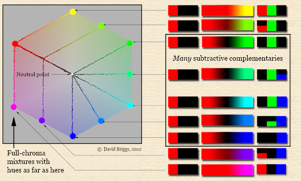
Figure 5.3.2. Subtractive mixing of a full-chroma additive primary with other "full-chroma" digital colours. Mixing paths displayed in plan view of YCbCr space, using the program ColorSpace by Philippe Colantoni.
Conversely, all full-chroma colours between two additive primaries have a single complementary, the third primary at full chroma, and therefore full-chroma subtractive primaries like "Monitor Magenta", which mix at full chroma with colours up to 120o away on either side, have only one complementary, directly opposite in hue . The resulting pattern of mixing paths is very distinct from that of a full-chroma additive primary like "Monitor Red" (Fig. 5.3.3).
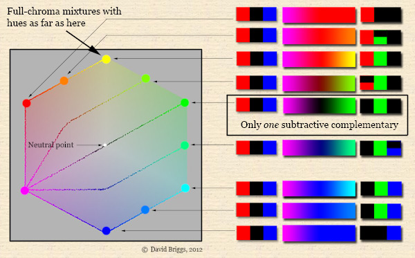
Figure 5.3.3. Subtractive mixing of a full-chroma subtractive primary with other "full-chroma" digital colours. Mixing paths displayed in plan view of YCbCr space, using the program ColorSpace by Philippe Colantoni.
Despite all of the additional complications involved, these two patterns seen in the simplest kind of subtractive mixing are still recognizable in the mixing paths of actual artist's paints (Fig. 5.3.4), as we will see in the next section.
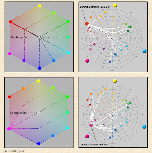
Figure 5.3.4. Comparison of ideal subtractive mixing patterns of full-chroma digital colours with mixing paths modelled for actual paints in the Munsell hue-chroma plane using the program drop2color by Zsolt Kovacs.
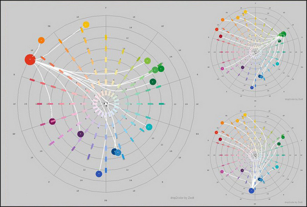
Figure 5.3.5. Mixing paths modelled for three paints close to the additive primary hues using the program drop2color by Zsolt Kovacs. For paint names see Fig. 6.3.6, Section 6.3.
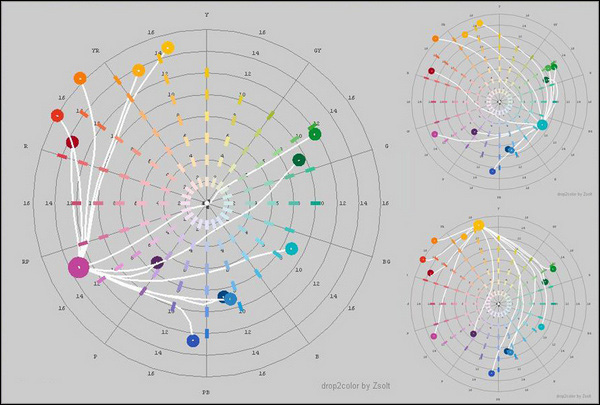
Figure 5.3.6. Mixing paths modelled for three paints close to the ideal subtractive primary hues using the program drop2color by Zsolt Kovacs. For paint names see Fig. 6.3.6, Section 6.3.
Modified June 26, 2012. For original (2007) page see here.
Next: Part 6: Colour Mixing in Paints