
my colour short course is
now offered online through
Australia's National Art
School in Sydney! There's
a choice of two sessions to
suit every time zone. LINK
Home
The Dimensions of Colour
Basics of Light and Shade
Basics of Colour Vision
Additive Mixing
- Additive primaries
- Additive mixtures
- Additive complementaries
- Additive-averaging & pointillist mixing
- Object colours
Mixing of Paints
Hue
Lightness and Chroma
Brightness and Saturation
Principles of Colour
Afterthoughts
Glossary
References
Contact
Links
NEXT COLOUR
WORKSHOPS

4.4 ADDITIVE-AVERAGING AND POINTILLIST MIXING
Additive-Averaging Mixing
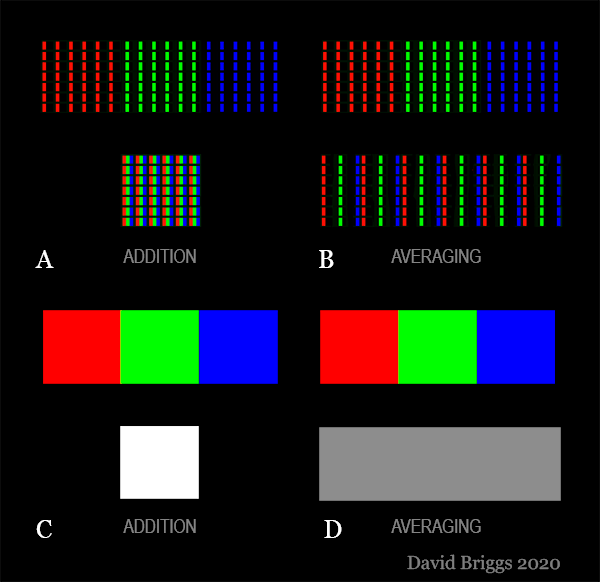
Figure 4.4.1. Microscopic (A,B) and macroscopic (C,D) views of examples of simple additive (A,C) and additive-averaging (B,D) colour stimulus mixing. Another example of simple additive mixing is seen in the overlapping of coloured light beams; another example of additive-averaging mixing is seen in spinning-disc mixture. (The grey rectangle in D shows the expected macroscopic appearance of stimulus C, but is produced in a different way, by dimming all of the RGB subpixels).
Up to this point we've been considering simple additive mixing, in which each light source adds its contribution to the amount of light reflected by or emitted from a given area. Examples include overlapping coloured spotlights and the contributions of the microscopic R,G and B subpixels to an area of a computer screen (Fig. 4.4.1A,C). In simple additive mixing the area lit by the mixture is necessarily brighter than areas lit by the components individually. On a computer screen an additive mixture of R,G and B lights at their maximum levels is the brightest area possible, and is normally perceived as the white object colour against which the colours of other areas are judged.
If the red, green and blue stimuli in Fig. 4.4.1A are not brought together in the same area but are instead intermixed over their total area, we still perceive an additive mixture of these components, in this case once again an achromatic or "white" light. However the quantity of light that was concentrated in the square in Fig. 4.4.1A is now spread across three times the area, so there is only a third as much light per unit area as in simple additive mixing, and so the mixture is perceived as grey (Fig. 4.4.1D). This kind of mixing has been given several different names, of which additive-averaging mixing will be used here. An additive-averaging mixture is necessarily less bright than a simple additive mixture of the same stimuli and is necessarily intermediate in brightness between the brightest and dimmest component stimuli.
The term optical mixing has long been used for processes in which two or more light stimuli in a given area can not be separately distinguished, so that the area is seen as a single colour. This name alludes to the idea that the coloured light mixes "in the eye" of the observer. This should not be taken to imply that the process is more subjective than other kinds of stimulus mixing; such effects can be photographed with a camera as well as seen first hand. Optical mixing can be either additive or additive averaging in effect, and can be either spatial, when the stimuli can not be distinguished because they are too small, or temporal, when the stimuli can not be distinguished because they are moving too fast. Another term available for these effects is partitive mixing, which is sometimes used in a broad sense for optical mixing including both additive and additive-averaging types, and sometimes in a narrower sense for exclusively additive-averaging optical mixing.
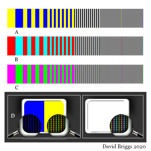
Figure 4.4.2. A-C, Additive-averaging mixing of additive complementaries. D, Microscopic view of stripes in A, compared with a white area on the screen.
Spatial additive-averaging mixing can be demonstrated on a computer screen if areas of different colours are interspersed finely enough that they can no longer be distinguished, as in Figures 4.4.2 and 4.4.3. At a sufficient viewing distance, as the stripes become narrower, the light from them is eventually seen as a single colour whose hue and saturation follow the usual results of additive mixing, but whose brightness is less than that of a simple additive mixture. Thus in Figure 4.4.2, where each pair of colours are additive complementaries, the resulting mixtures are achromatic or "white" light, because the total numbers of R,G and B phosphors glowing are equal in each case. However, because only half the number of phosphors are emitting light as in an area of white screen, the mixture is seen as grey, not white (Fig. 4.4.2D). Although emitting half as much light as a white area, the grey is lighter than middle grey on on a typical lightness scale because these are nonlinear with respect to energy.
Spatial additive-averaging mixing is also experienced in an image made of light-reflecting coloured dots that are too small to be distinguished visually, for example in a pointillist painting viewed at a much greater distance than the intended viewing distance. The effect is perceived as additive-averaging rather than simple additive because the mixed areas are judged relative to the brightness of a similarly illuminated white area. (We would similarly judge the RGB mixtures on a computer screen as additive-averaging if we compared them with a hypothetical screen on which all of the subpixels emit white light, but this is irrelevant). Spatial additive averaging mixing is involved in all printing processes that involve finely interspersed dots of ink, although such processes also involve subtractive mixing wherever the dots of ink overlap.
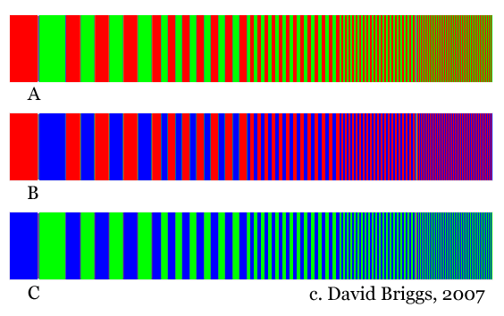
Figure 4.4.3. Additive-averaging mixing of additive primaries.
Similarly in Fig. 4.4.3, the mixtures have the hue and saturation but not the brightness and chroma of the colours that would be expected from simple additive mixing.
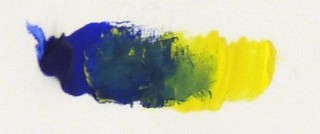
Figure 4.4.4. Above: spinning disc displaying temporal additive-averaging mixing of additive complementaries, ultramarine blue and cadmium yellow light. From the point of view of the human visual system the spinning disc reflects achromatic (white) light, but less white light than a white disc would reflect, so the disc is seen as grey. Below: physical mixture of ultramarine blue and cadmium yellow light paint. The subtractive component involved in paint mixing yields dull green and yellow green colours.
Spinning discs are a well-kown example of temporal additive-averaging mixing. In Fig. 4.4.4, very little short-wavelength (violet and blue) light is reflected from the area of the yellow disc, and little middle and long-wavelength light (individually red, yellow and green) light is reflected friom the area of the ultramarine disc, so that the light reflected from the two areas is complementary in additive terms. When the areas of the two colours are correctly adjusted the light reflected from the spinning discs is achromatic or white, but the amount of white light is less than a white disc would reflect, and the disc is therefore seen as grey. You may already know that a physical mixture of these paints would look green rather than grey; but this difference is anomalous only if you assume (wrongly) that it is the colours blue and yellow that are mixing. Don't forget that the blue and the yellow are perceptions in our minds and do not exist or mix in paints or in light.
We'll see that additive-averaging mixing, combined with subtractive mixing, plays an important role in physical mixing of all paints except those that are entirely transparent (see Part 6).
Pointillist Mixing
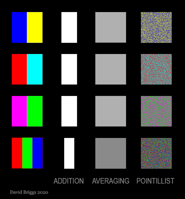
Figure 4.4.5. Simple additive, additive-averaging and pointillist mixing of the colour stimuli on the left. In pointillist mixing, unlike additive-averaging mixing, the component stimuli remain visible at the intended viewing distance, creating a soft and lustrous effect.
Another kind of colour stimulus mixing that is often equated with additive-averaging mixing, but is actually quite distinct, is pointillist mixing, in which very small coloured areas are finely interspersed but are large enough to remain generally perceptible at the intended viewing distance (Fig. 4.4.5). The effect is named after the technique of the Neo-Impressionist painters beginning with Seurat. In pointillist painting the interspersed dots of paint at the intended viewing distance typically produce a soft and lively "lustre" not obtainable using uniform paint mixtures.
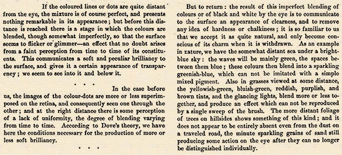
Figure 4.4.6. Ogden Rood describing the effect of what would later become known as pointillist mixing, in his influential textbook on colour science for painters, Modern Chromatics (1879, pp. 280-281).
The technique was recommended for this effect and also as a way of evoking the appearance of natural landscapes by Ogden Rood in his book Modern Chromatics (1879), which is known to have been studied by Seurat (Fig. 4.4.6).
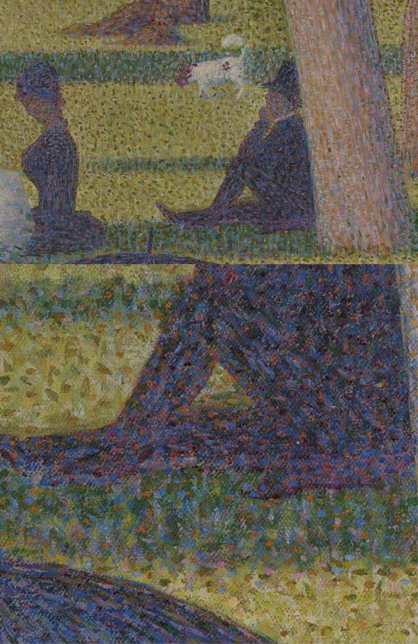
Figure 4.4.7. Details of Seurat's La Grande Jatte. Image credit: Google Arts & Culture. Many of the dark spots are now believed to be degraded zinc yellow.
Elsewhere in his Modern Chromatics Rood demonstrated experimentally that optical (spinning disc) mixtures of paints always had greater "luminosity" (meaning only that they were higher in lightness) than physical mixtures of the same paints. This observation was perfectly well-founded in itself, but came to be widely misinterpreted to mean that colours obtained by optical mixing are lighter and/or more intense than any that can be obtained by physical mixing of paints. This error is sometimes attributed to Rood or to Seurat, but falsely in both cases. As can be seen in these details of La Grande Jatte (Fig. 4.4.6), Seurat uses only very simple pointillist mixing to obtain his highest chroma colours (e.g. the sunlit grass - in which by the way there is no ill-advised attempt to mix the green from dots of yellow and blue!), and little or none to obtain his lightest colours (e.g. the brightest white of the dog). Instead, Seurat uses his most elaborate pointillist mixtures in his darkest areas, which therefore sparkle with traces of intense colour and display the "soft and peculiar brilliancy" described by Rood. Seurat reportedly chose the colours of the dots using the concept of “spectral decomposition”, for example the areas of shaded grass are represented using numerous dots of dark green for the object colour of the grass, combined with dots of blue for the hue of skylight, dots of purple for the complementary of the adjacent sunlit grass, and dots of yellow-orange for the hue of reflected sunlight.
Page modified March 30, 2020. Original text here.