
my colour short course is
now offered online through
Australia's National Art
School in Sydney! There's
a choice of two sessions to
suit every time zone. LINK
Home
The Dimensions of Colour
Basics of Light and Shade
Basics of Colour Vision
Additive Mixing
Subtractive Mixing
Mixing of Paints
Hue
Lightness and Chroma
Principles of Colour
Afterthoughts
Glossary
References
Contact
Links
NEXT COLOUR
WORKSHOPS

Please note: The pages forming Part 8 were part of the original Dimensions of Colour site uploaded in 2007 and have not been updated recently. They are left here for the moment because some of the diagrams have been linked to by other sites or reproduced in publications. For much more recent discussions of lightness and chroma please see:
Section 1.3 The Dimensions of Colour: Lightness
http://www.huevaluechroma.com/013.php
Section 1.5 The Dimensions of Colour: Chroma
http://www.huevaluechroma.com/015.php
HUE-CHROMA-LIGHTNESS COLOUR SPACES
A colour wheel can represent relative chroma on a radial axis and hue by position around the wheel, but a third dimension is needed if all object colours are to be represented. The simplest way to do this is to add a third axis representing relative lightness at right angles to the colour wheel, creating a simple solid such as a sphere or a symmetrical double cone. A cylinder would also be possible, but would not represent the convergence of object colours as they approach black and white respectively. Examples of a spherical colour space of this type include that of Otto Runge, published in 1810, and the one devised by Johannes Itten (Figure 8.6). An example of symmetrical double cone arranged on this principal is the HLS digital colour model. [In the symmetrical double cone in the colour classifications by Ostwald (Figure 8.7) and the Scandinavian Natural Colour System colours are arranged according to scales of black/white/colour content, and the vertical dimension is not intended to represent lightness].
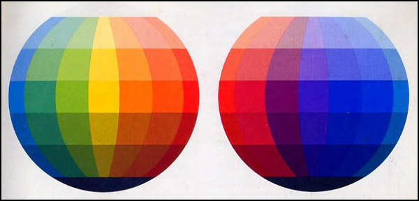
Figure 8.7 . Colour sphere of Johannes Itten (1961).
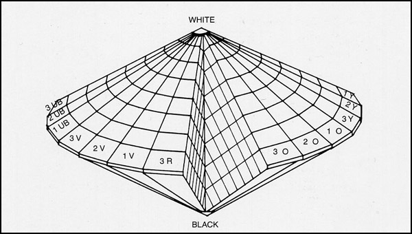
Figure 8.8. Symmetrical double cone colour solid by Ostwald (Bond and Nickerson, 1942).
One shortcoming of both the sphere and the symmetrical cone conceptions of hue-lightness-chroma spaces is that, as we have just seen, different hues reach their maximum chroma at different lightness levels. Putting all of the "full" colours on the equator of the solid ensures that the vertical dimension does not represent absolute lightness. Consequently neither the Runge-Itten sphere nor the HLS digital model is a true hue-chroma-lightness space. If the vertical dimension of the solid is to represent absolute lightness, then we need in some way to tilt the plane of "full" colours through space, so that the yellow occupies a high position opposite light grey and the blue occupies a low position opposite dark grey.
This requirement can be satisfied most simply in a skewed double cone, a solution first suggested by Kirschman (1896) (Figure 8.9A). Arthur Pope (1922, 1931) described in detail a similar double cone space, implicit in, though not actually illustrated in, the colour system of Denman Ross (Figure 8.9C). Both of these double cone solids are simple conceptual models in which chroma is normalized, so that they have a simple circular appearance in plan view. Following Ross, the Pope solid uses a hue circle based on the traditional artist's colour wheel, but analogous solids based on hue circles of psychological, additive or pigmentary complementaries could easily be visualized. A simple conceptual model of this sort is valuable for many purposes of practical painting.
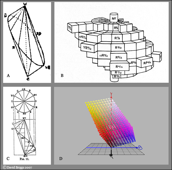
Figure 8.9. Representations of hue-chroma-lightness space by (A) Kirschman (1896) (flipped), (B) Munsell system (Bond and Nickerson, 1942), (C) Pope (1922) and (D) YCbCr spaces, all viewed from similar angles.
The Munsell system uses dimensions of absolute lightness and chroma, and so has an irregular, tree-like appearance, reflecting the fact that the maximum chroma obtainable in object colours varies markedly for different hues.
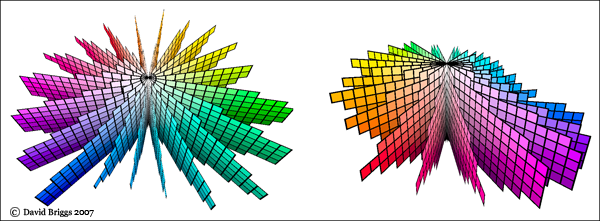
Figure 8.10. Two views of the Munsell colour space generated using a programme by John Kopplin (http://www.codeproject.com/directx/d3dmunsell.asp)
RGB (screen) colours have a distinctive geometry in hue-lightness-chroma space related to the way they are generated. Among full-chroma screen colours, the cyan, magenta and yellow secondaries are all lighter than their adjacent primaries: L = 98 for yellow, 60 for magenta and 91 for cyan, compared to 88 for green, 54 for red and 30 for blue. These differences can be accounted for by the fact that in the secondary colours, pixels of both the adjacent primaries are glowing. Magenta and cyan consequently disturb the steady fall in lightness from yellow to violet-blue on both sides of the hue circle (Figure 8.9D, 8.10).
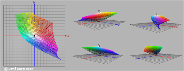
Figure 8.11 . RGB colours arranged in Lab colour space, using the program RGB Cube by
Philippe Colantoni.
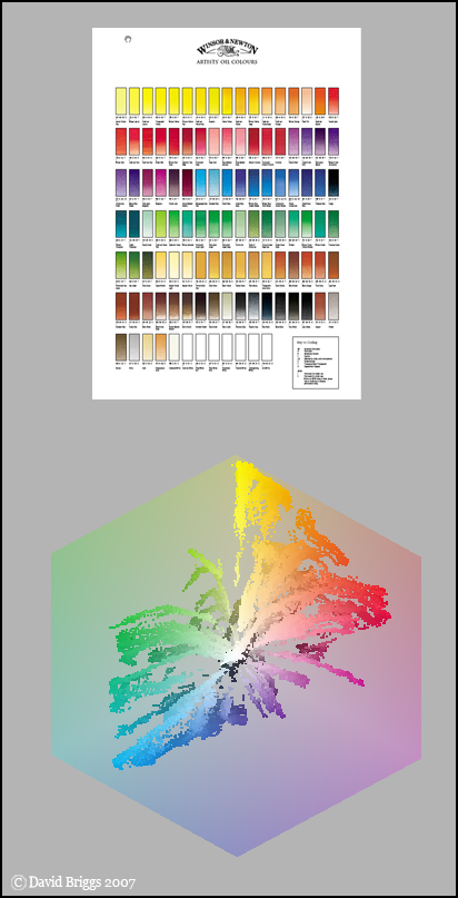
Figure 8.12. Colours of about 100 coloured pigments from a Winsor and Newton colour chart (pdf version).
????????